Landmark Classification & Tagging for Social Media

Skills: CNN, Pure PyTorch & FastAI, Transfer Learning, Image Processing, CLI

Models: ResNet34 & SqueezeNet

Introduction

Photo sharing and photo storage services like to have location data for each photo that is uploaded. With the location data, these services can build advanced features, such as automatic suggestion of relevant tags or automatic photo organization, which help provide a compelling user experience. Although a photo's location can often be obtained by looking at the photo's metadata, many photos uploaded to these services will not have location metadata available. This can happen when, for example, the camera capturing the picture does not have GPS or if a photo's metadata is scrubbed due to privacy concerns.

If no location metadata for an image is available, one way to infer the location is to detect and classify a discernible landmark in the image. Given the large number of landmarks across the world and the immense volume of images that are uploaded to photo sharing services, using human judgement to classify these landmarks would not be feasible.

The project was initially part of the Udacity's Deep Learning Nanodegree path which was then remastered to be a standalone example. There were further improvements in parameter exploration, model architectures breakdown and comparison, as well as re-implementation using the famous framework FastAI. It can further be used with CLI to get the landmarks classified directly or train your own models (all models supported by FastAI and PyTorch). Please see the GitHub repository for this project to learn more.

Data

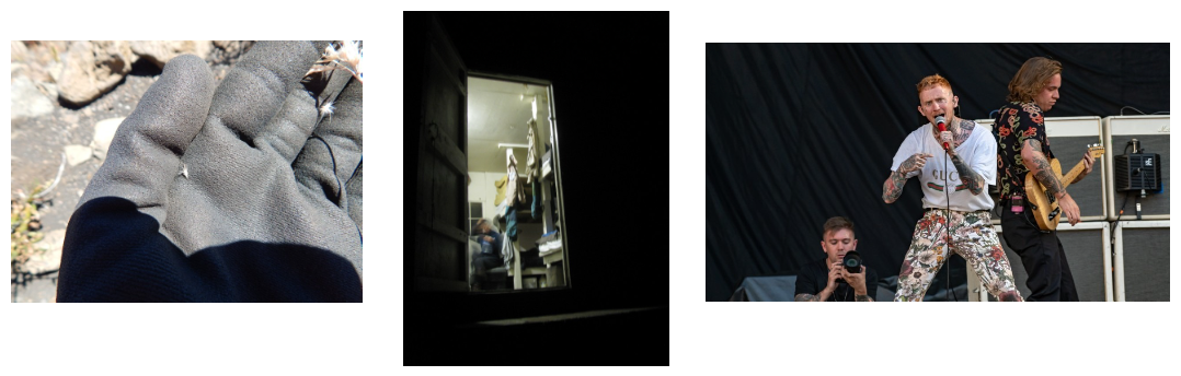
The data used in this project is a subset from Kaggle's Google Landmarks competition. It contains 5000 images from 50 different locations worldwide. The dataset includes a good number of irrelevant images that show people, gears, and other objects as shown in Fig 1. These images can potentially mislead the model to wrongly hyperfocus on irrelevant elements. To test the model's capabilities, I decided to leave the images untouched. Later on, we will look at the misclassified images, their statistics, and decide whether they had a weight on final predictions.

Implementation

There are two different approaches the project was conducted in: vanilla PyTorch and FastAI. Pytorch is a machine learning/deep learning library that combines efficiency and speed with help of GPU accelerators [1]. FastAI is a deep learning library built on top of PyTorch that allows users to quickly put their ideas into a working state. It provides low-level components that can be mixed together to provide more efficiency and reliability [2]. The choice to use pure PyTorch was driven by the desire to build data preprocessing, training, and validation pipelines from scratch. FastAI was chosen to take advantage of pre-made low-level components and built-in capabilities to find global minima on its own; thus checking which approach gives better performance. Both approaches were tracked locally using NVIDIA GeForce GTX 1650 GPU accelerator.

Models

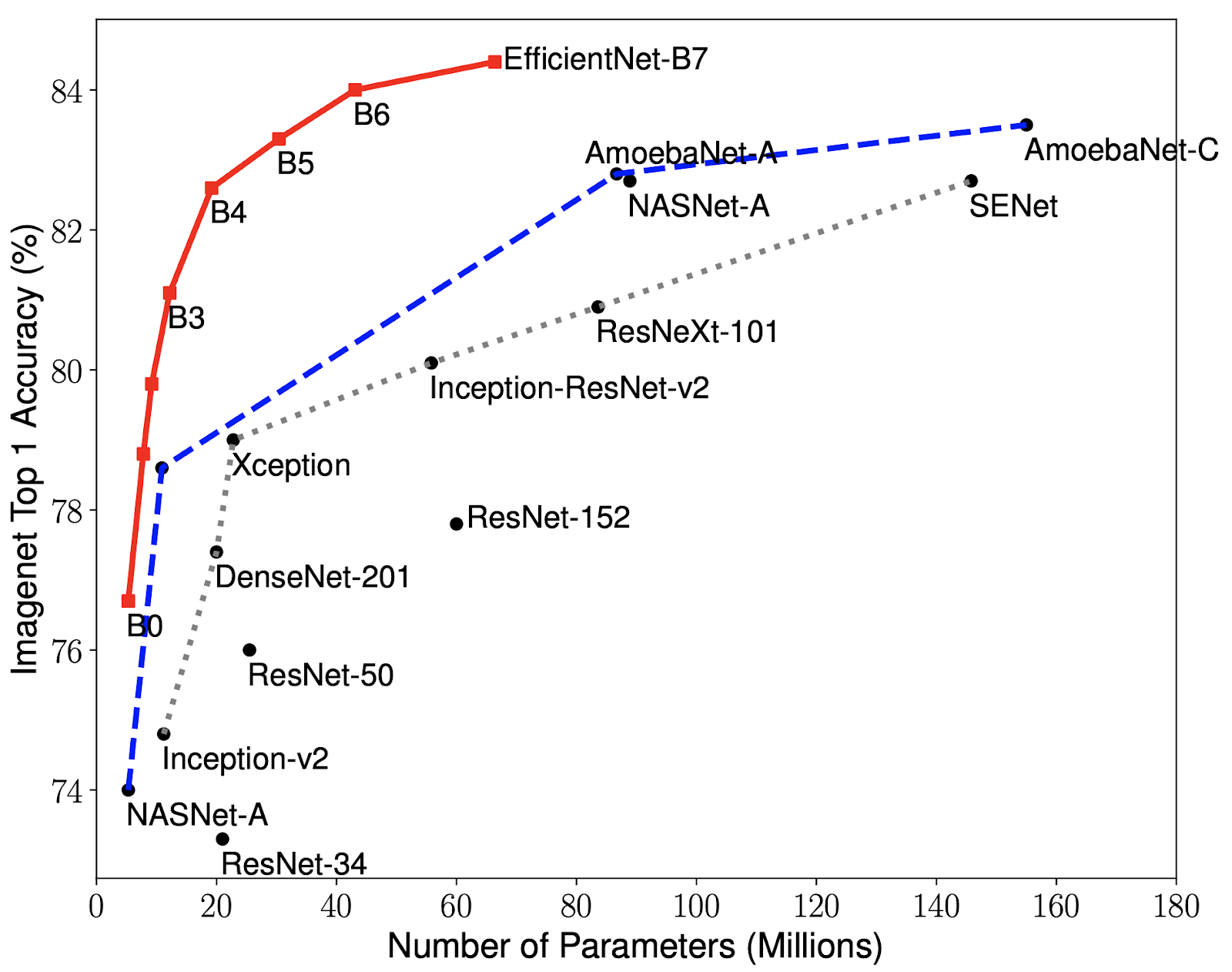
There is a vast number of architectures that stored over 70% accuracy at ImageNet's TOP-1 classification such as EfficientNet-B7 (with 70 million parameters and ~85% accuracy), ResNet-34 (with 20 million parameters and ~72% accuracy), DenseNet-201 (with 20 million parameters and ~77% accuracy). A variety of architectures with the number of parameters and accuracies can be seen on Fig. 2. The choice for this project was to use two different models that are present in the figure below, ResNet34 and EfficientNet-B7. However, FastAI does not support the second. Therefore, the two models selected for experimentation are ResNet34 and SqueezeNet.

ResNet34

Deep Residual Networks were first introduced in 2015 by Microsoft's researchers Kaiming He, Xiangyu Zhang, Shaoqing Ren, and Jian Sun. The central idea of which was to introduce a residual learning framework to ease the neural network training that were much deeper than the preceding architectures. The main issue with having too deep models is the problem of vanishing or exploding gradients. This happens during the backpropagation process where a model calculates partial derivatives of the error function which get multiplied at each training iteration. If the update in weights is too small, they do not change. Alternatively, in the case of exploding gradients, the behavior is reversed. The weights become too large too fast.
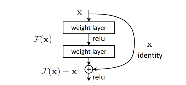
Even though the aforementioned issue has gotten some workarounds such as intermediate normalization layer [3, 4, 5, 6], this paper introduces a different approach by changing the underlying mapping $F(x) := H(x) - x$ to $F(x) + x$ . This is done by adding the "shortcut" connections in the feedforward process. These shortcuts skip one or more layers by performing identity mapping, whose outputs gets added to the output of the stacked layers [7]. By doing so, the model does not learn new parameters nor get more complex.

SqueezeNet

SqueezeNet was introduced in 2016 by Stanford's researchers Forrest Iandola, Song Han, Matthew Moskewicz, Khalid Ashraf, William Dally, and Kurt Keutzer. The architecture took a different approach from all the existing architectures by introducing a lightweight model that could be easily deployed and can be compressed to 0.5MB [8]. Having such a weight made possible to be exported to autonomous cars and other applications where memory is limited. SqueezeNet achieves the same accuracy as AlexNet while having 50x fewer parameters.

Results

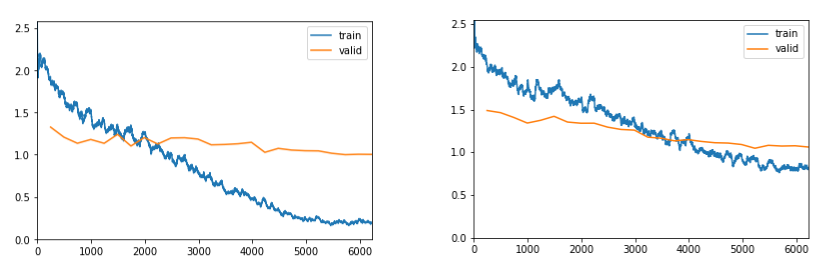
Both models were trained for 25 epochs with focus on F1 score, both scored over 70% and roughly had the same training time, 71 and 75 minutes respectively. ResNet34 got 79% accuracy/F1 score, whereas SqueezeNet scored 73% on both metrics. Surprisingly, each model misclassified different sets of images. The first confused Mountain Rainier with Banff National Park the most (5 times), whereas SqueezeNet misclassified it twice only. The biggest confusion happened between Yellowstone National Park and Machu Picchu (4 times).

Future Work

The above image shows that validation losses is somewhat flat on both occurrences. It is important to understand why such behavior is present. Furthermore, a lot of things can be done to improve the model's performance. First and foremost, go through the dataset one-by-one and remove all unnecessary images that do not help identify the landmark. Second, increase the number of images in training set to cover the places from different angles, seasons, with and without people; it is important to give the model enough data to focus on important aspects. Third, dig into the misclassified images and find correlations. This can be further explored using GradCam to see where the model focuses its attention. Forth, consult novel approaches in CNN image classification, there might be good insights to train such models. Last, look into data-centric techniques to clean data appropriately.

References

[1] Paszke, Adam, et al. "Pytorch: An imperative style, high-performance deep learning library." Advances in neural information processing systems 32 (2019).
[2] Howard, Jeremy, and Sylvain Gugger. "Fastai: a layered API for deep learning." Information 11.2 (2020): 108.
[3] Y. LeCun, L. Bottou, G. B. Orr, and K.-R. M ̈uller. Efficient backprop. In Neural Networks: Tricks of the Trade, pages 9–50. Springer, 1998.
[4] X. Glorot and Y. Bengio. Understanding the difficulty of training deep feedforward neural networks. In AISTATS, 2010.
[5] A. M. Saxe, J. L. McClelland, and S. Ganguli. Exact solutions to the nonlinear dynamics of learning in deep linear neural networks. arXiv:1312.6120, 2013.
[6] K. He, X. Zhang, S. Ren, and J. Sun. Delving deep into rectifiers: Surpassing human-level performance on imagenet classification. In ICCV, 2015.
[7] He, Kaiming, et al. "Deep residual learning for image recognition." Proceedings of the IEEE conference on computer vision and pattern recognition. 2016.
[8] Iandola, Forrest N., et al. "SqueezeNet: AlexNet-level accuracy with 50x fewer parameters and< 0.5 MB model size." arXiv preprint arXiv:1602.07360 (2016).